3 act task: mowing the lawn
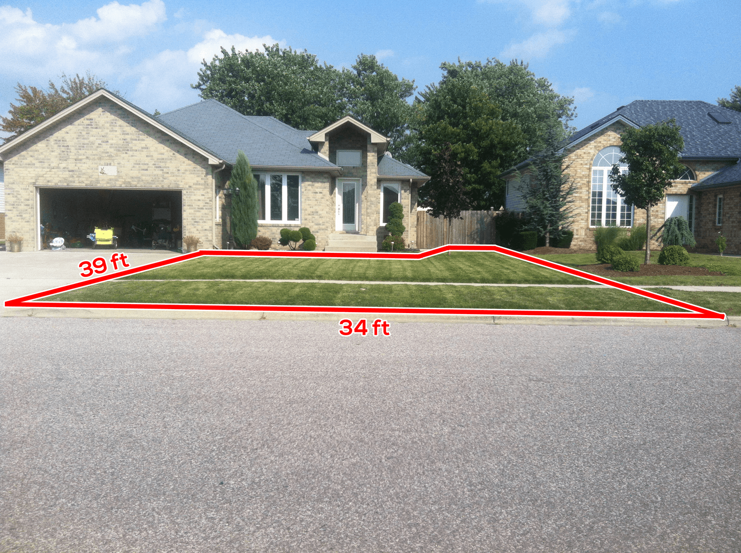
We worked on composite area and pythagorean theorem today in grade 9. There’s a good 3 act task called mowing the lawn. It starts with a lawnmowing video to pique the interest, and get questions flowing.
Next, another video, with a timer, and also dimensions given for the mower and for the lawn

I usually wait until they ask how wide the mower is. Often we get so bogged down with area calculations that we forget the mower has a width too!
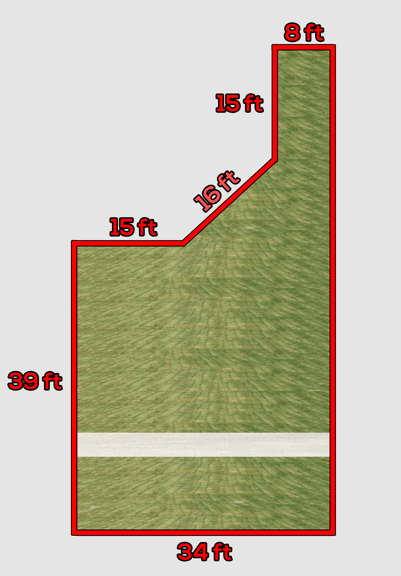
We then worked really hard for quite a while to calculate the area of the lawn and how long it would take to cut.
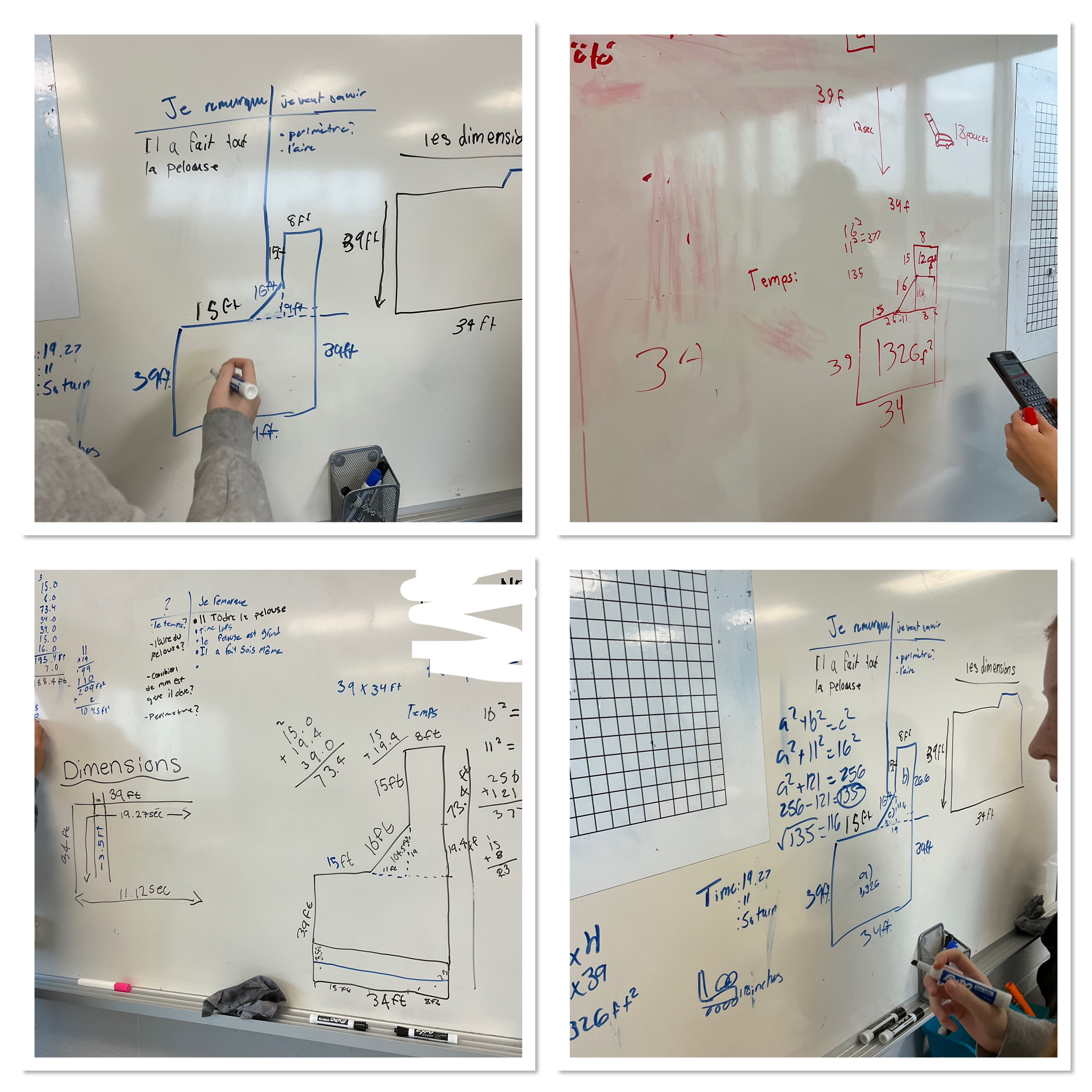
Some common errors I’ve noticed were in applying pythagorean theorem to calculate a triangle leg vs hypotenuse. Also some students struggled with 18 inches being 1 foot 6 inches which is 1.5 feet (not 1.6 feet). Others struggled with how to use unit rates that would be helpful like how many seconds it takes to cut one square foot of lawn. That can then be scaled up to figure out the time to cut the entire area of the lawn. There were good conversations about how many pieces to break the yard up into, and if it mattered if he mowed in a spiral pattern or back and forth in rows.
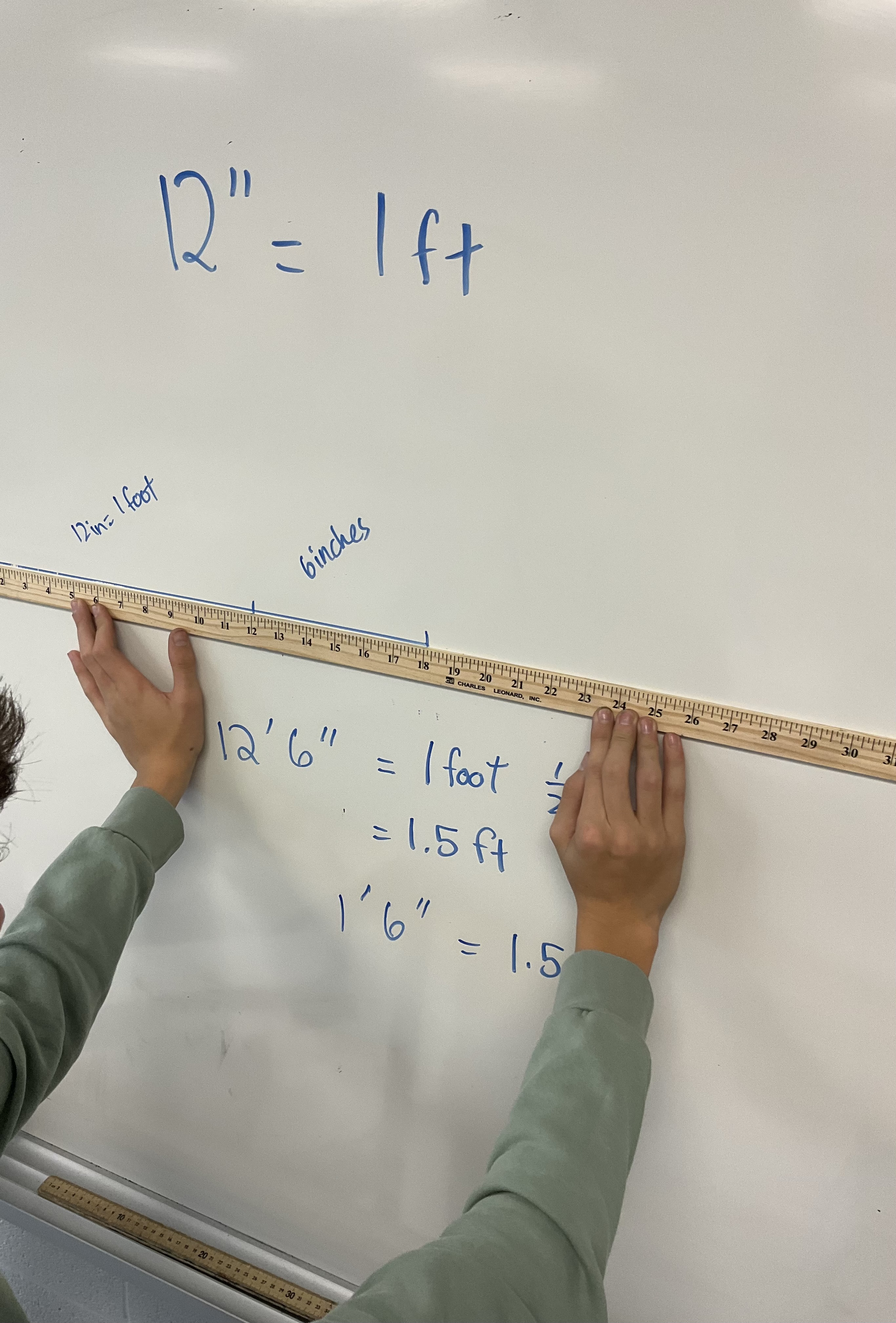
I’m thankful that our meter sticks are also yard sticks, so we can work in inches and feet when we need to.
In the end we watched the whole video to see the answer. Watch for motion sickness!
We did a lot of calculating and reasoning today. We need to work on our communicating…that will be our next step.
Area of Regular Polygons
Today in MFM2P we looked at area calculations, to review and activate prior knowledge and then apply it to some new challenges.
Groups started with a sheet that led them through some calculations. They worked collaboratively in pairs or groups of 3 to go through these early questions. It’s interesting to me what ideas stick (area=basexheight seemed to be in their memory, but they had forgotten the word parallelogram)

We talked about how you could find the area of the triangle pieces and the rectangle piece and add them up, but ALSO how you could slide the triangle piece over and create a rectangle. The formula for area is still base times height, but we have to remember that height is perpendicular to base always.
Next in the sequence was to look at a right angle triangle and relate that formula to what we know about rectangles. This is half a rectangle, so the area should be (1/2)(base)(height).
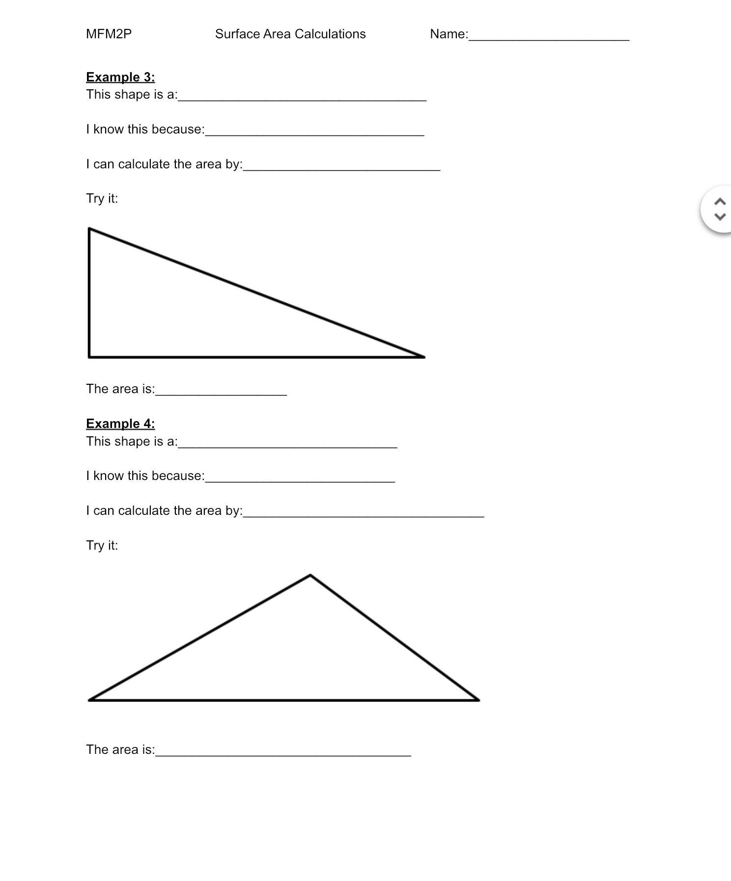
The bottom triangle has the same formula for the same reasons. We can draw a rectangle around the triangle. Looking at each side, half of the rectangle is in the triangle, and half is not.

Next we branched out to regular polygons. This was a bit of a leap, it is so visually different that some students had a moment of giving up. It’s neat to see how we can make a visually different figure appear to be a parallelogram by using scissors!

We drew lines from the corners to the middle, then cut out along those lines. We could fit them together upright and inverted to build a parallelogram. If we cut one of the triangles in half and slide it over we would have a rectangle. The base would be half of the perimeter of the shape. For this dodecagon we can see that there are 6 of the “edge segments” that make up the top and bottom sides of the parallelogram. The height of the shape is the same as the height of one of the triangles. This distance is called the apothem (not an important word, but it’s like the radius of the non-circular shape).

We can make any regular polygon into a rectangle to calculate its area. We can explore how this helps us understand circle areas, but we’re not there yet. This also sets the stage to calculate volume of any regular polygon based prims (and later pyramids).
M&Ms task
Today my grade 9 class tackled the M&Ms task.

Students counted, dumped, removed all the “M” side up candies, then counted, dumped and repeated the process. They added to a data table as they went, and noted that there was a big drop at first, and less and less of a drop as it went on. Some saw the connection to the drop being about half each time, which was neat to see. Again, we noticed that 8-12 candies had no M printed at all, so we never ended up eliminating all of them.

Groups created graphs and saw that the pattern was not linear, but looked like a decreasing curve. They made curves of best fit to model the data.
We talked about how to make an equation to generalize what we saw happening. We know that to find half of a number we can divide by 2 or multiply by 1/2. If we find half of THAT number then we’d have to multiply by 1/2 again. We showed that in our table of values for an example case of starting with 160 candies.

We could use our exponent knowledge to help us build the equation. This type of modelling will be important when we look at compound interest later on.
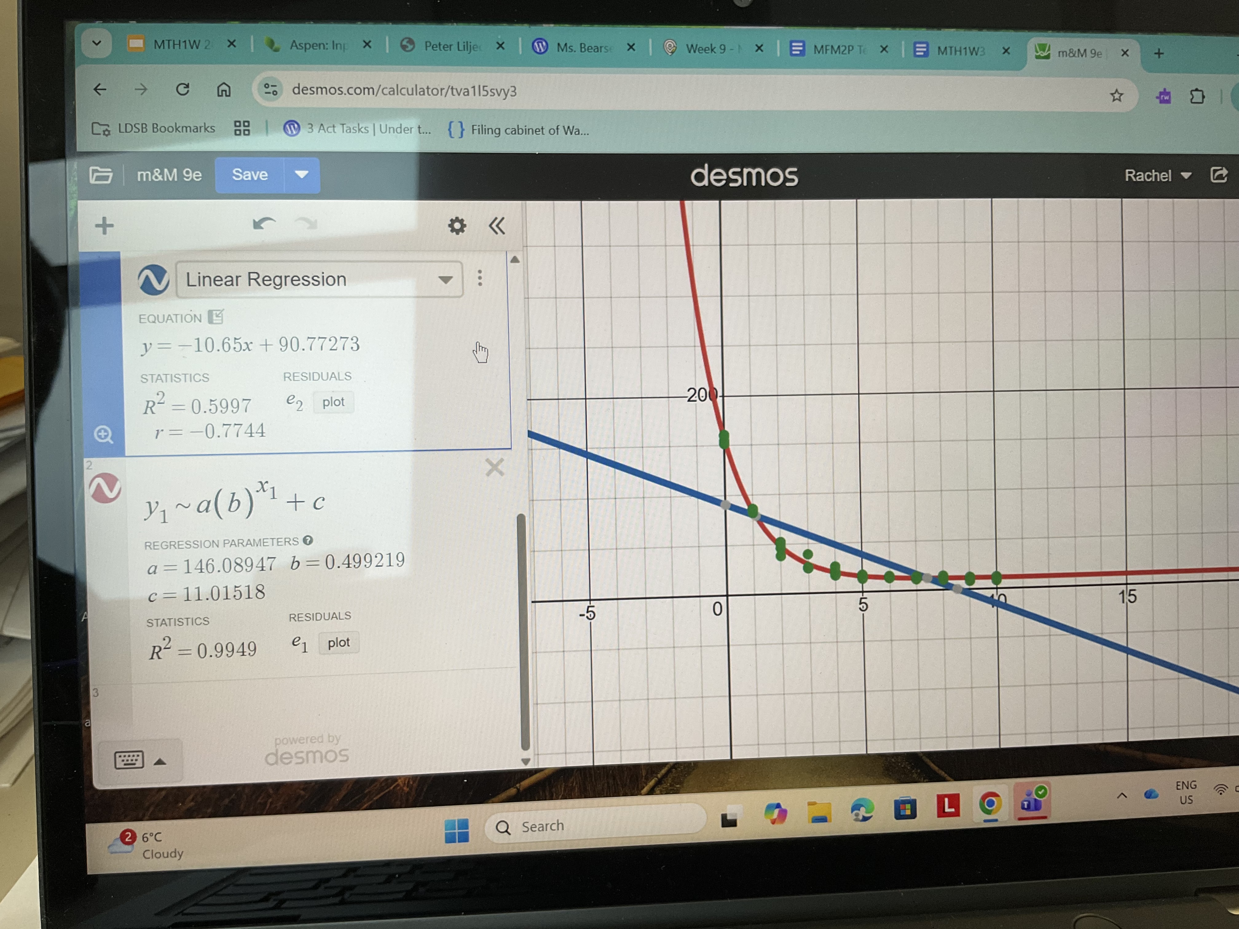
Finally we modelled the class data on desmos and looked at how to do a regression. We followed the same model as we created together, but left the initial value as “a”, the base of the exponent as “b” and the vertical shift for the horizontal asymptote as “c”. We talked about the R squared value and how it’s a really good fit. We compare this to the linear regression that Desmos does. We noticed that the linear regression has an R squared of 0.59 which is not as good a fit.
This was a nice way to spend a Hallowe’en Friday, eating some candy and making some graphs, and learning some pretty sophisticated modelling skills.
Equations to Graphs via Visual Patterns
Today I had the pleasure of running a task in a colleague’s grade 9 math class. We’ve been working on patterning, pattern rules (equations) and graphs. Today the goal was to start with an equation and end up with a graph, but we used visual patterns as the intermediate step.
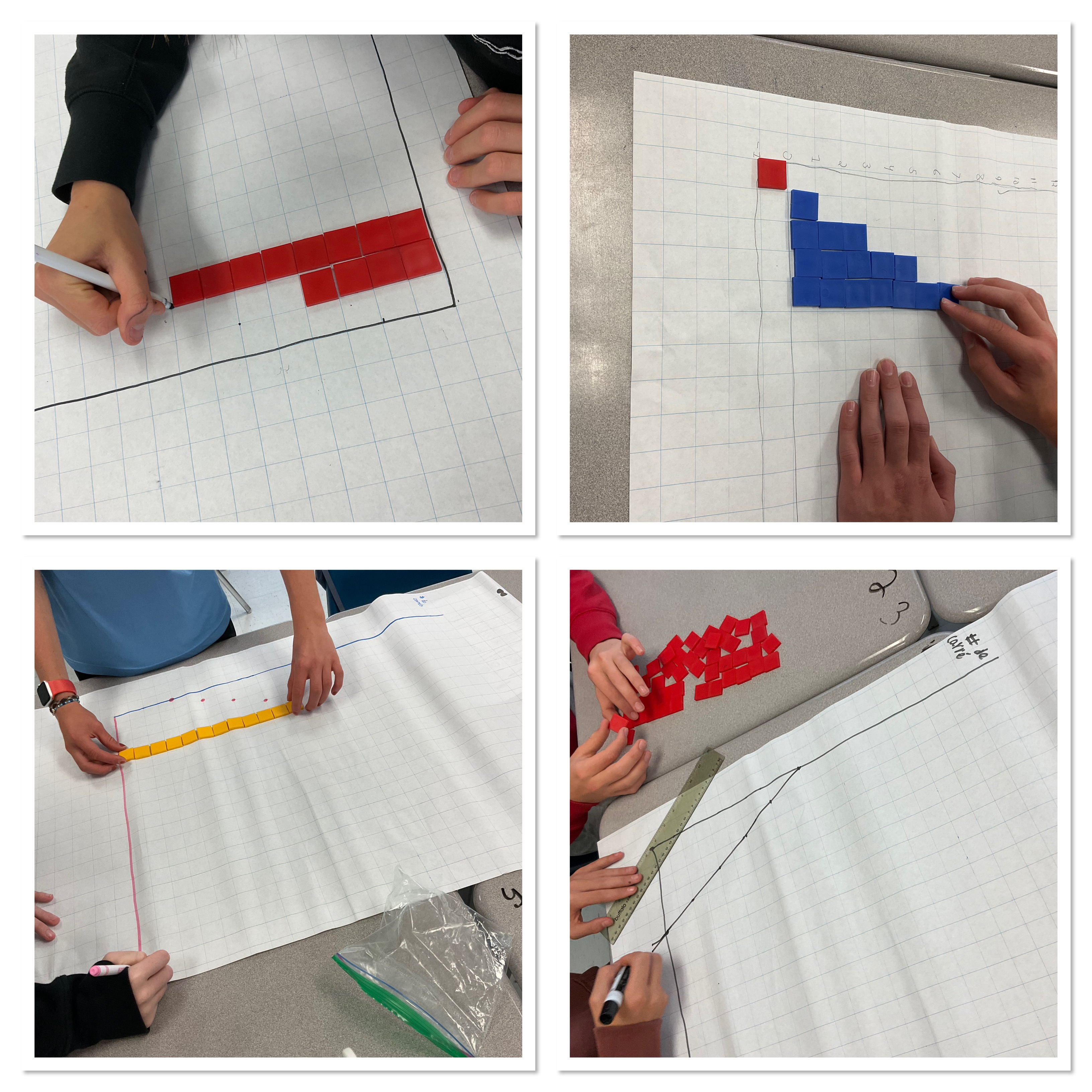
Each small group of students were given an equation (pattern rule) and were challenged to build figure 0, figure 1, figure 2, figure 3 and figure 4.

Next they brought their tiles from each figure number one at a time to build columns on a graph. All the blocks from figure 0 were lined up on a tower along the y axis, all the blocks from figure 1 were lined up in a tower next to it etc.

Dots were placed at the top left of each column of blocks to indicate the height of the column, and later we removed the tiles and joined the dots to make a line.

Next students were given a different pattern rule and we did the same thing again, making a new pattern, new columns of blocks, and then new points and a new line, with a different colour marker.

Some groups did more than 2 graphs. Others did just 2. Some had some misplaced points which we left on the graphs and then used them for points of discussion later.

We got groups to clean up and then we posted the papers on the wall to use as our consolidation. Now, there is a bit of an art to getting a good consolidation on these tasks. It starts with pairing up the equations well to get something to discuss. I made sure to have some lines with positive slopes and negative slopes, some lines that had the same y intercept, some lines that would intersect with each other. Some lines with positive and negative y intercepts, and some parallel lines. The next part about the consolidation is to meet the class where they are at. Many students were comfortable talking about all of the graphs being lines, or about them being increasing (growing patterns) or decreasing (shrinking patterns). Once we got all of those ideas up on the pages we started looking at more similarities and differences among the lines, introducing new vocabulary when possible.
I get the class to do a call and response of “parallèle” “même pente” which I think is fun, and it helps reinforce the idea that parallel lines have the same slope.


We took a bit of a break and watched some of my favourite life changing math videos:
Next we consolidated the final graph. We showed more detail about the slope and how we can use various points to show the slope triangle, and the fraction can be simplified. We also looked at how the point of intersection is on both lines, so when you sub in the x ans y values it makes the equation true.

It was a really productive class, and quite fun to collaborate with my colleague and introduce her to this task.
M&Ms task
Today I had the pleasure of working with a grade 11 math class who have been studying exponential growth and decay.
we started by sanitizing our hands because we were going to be touching candy which we wanted to eat later.
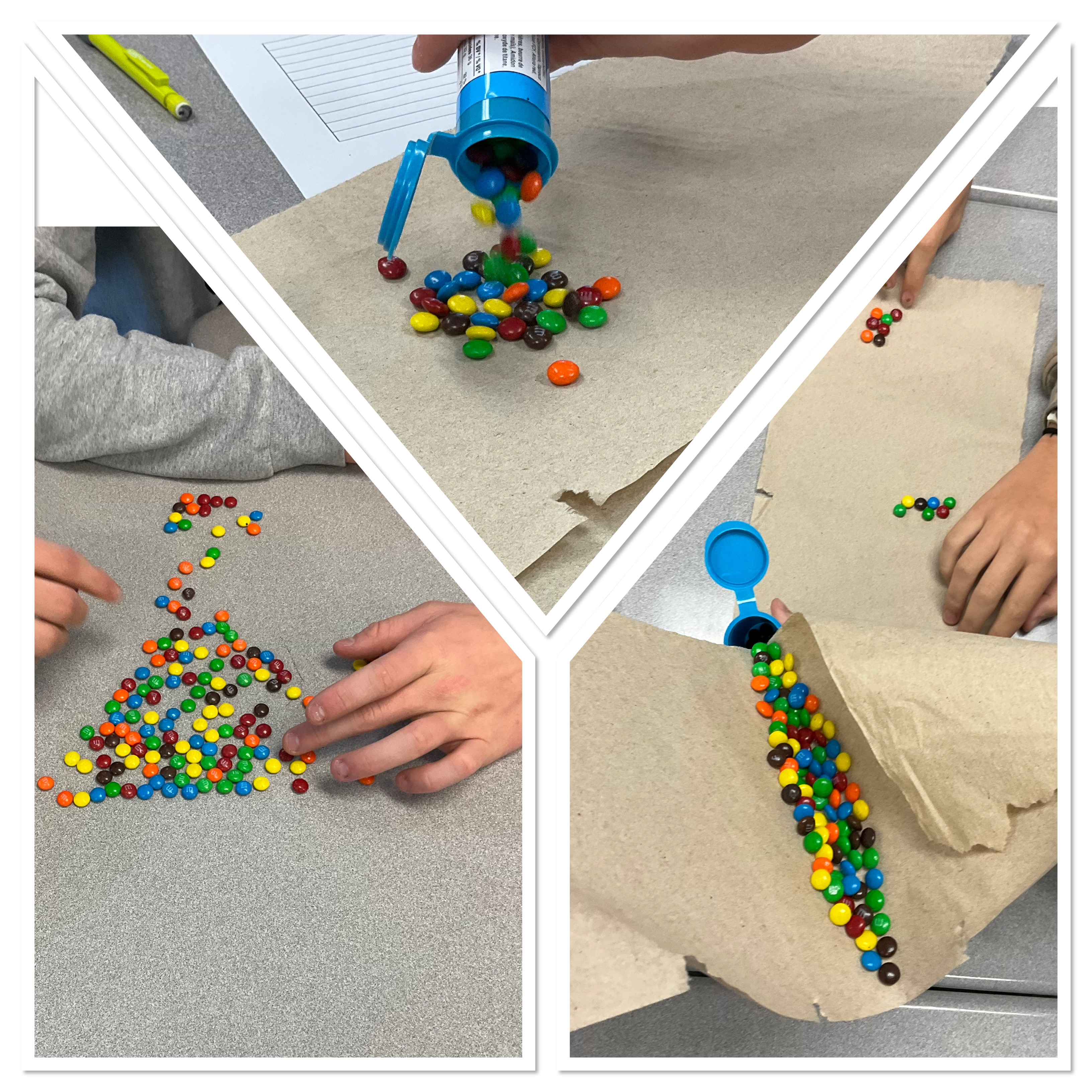
Each group got a tube of mini m&ms. They needed to count how many were there to start with, and add information to a data table.

Next we put all the m&ms into the tube and dumped them.
We eliminated (ate) all the ones with the M side up, and counted the remaining ones, added that to the data table, and repeated until we were done 10 repeats.
Next we made graphs using our data table, and tried to make sense of what type of relationship we saw, and what equation would model the data.

We noticed that the number of m&ms remaining dropped fast at first, and slowed as we continued. Some groups noticed that they had 8-13 remaining, even after repeating the process 15 times. It turns out some m&ms didn’t get printed!
We noticed that there was a horizontal asymptote that appeared. The graphs were showing exponential decay. Since we removed about half the m&ms each time, or since there was a 50-50 chance of them landing m side up, we used 0.5 as the base of the exponent. We know that the x will be the exponent. We needed a vertical shift to have the horizontal asymptote in the right spot, and we used the “a” value, a vertical stretch to get the y intercept in the right spot. Knowing that anything raised to the exponent 0 is 1 is very helpful!

Next groups got computers and put their data into desmos and used the extrapolations available there. We noticed that if you use the exponential regression that desmos has from their drop down menu that the horizontal asymptote is at the x axis. To do a more precise regression you can type it in. This graph is the aggregate of all of the class data, shown on one graph.

It’s important to remember the subscript 1 which ties the x and y values to the data table with x1 and y1. The ~ indicates that a regression is to be done, and there will be values given for each of the parameters provided in the equation. The r squared value will also be given.
It was neat to see the connections the students were making to their prior knowledge. They understood what the asymptote would represent in this situation, and how the base had to be a value between 0 and 1 since it was a decay situation. I was impressed at how well the data from the experiment worked out, and how clear it was that we were dealing with exponential decay.
I had debated having the students eat the m&ms without the m showing, but I think that they would have missed out on a rich conversation about the horizontal asymptote being representative of the “defective” candies that didn’t get printed. The task could be done with skittles as well, but the mini m&ms work well since they are small so each group starts with a large number, and can see the decay rather dramatically at the start.
Three Act Tasks
Today in grade 9 we did 2 different 3 act tasks to explore linear relations. The first one we did was Crazy Taxi.
We watched act 1 and we noticed and wondered for a bit. There’s lots going on! We talked about price and speed and distance…then we watched this video to see more and to get prompted with what to calculate. We looked at what the cost would be for a trip that was 30km.

Students used several representations, making tables, and equations and graphs to solve the problem.
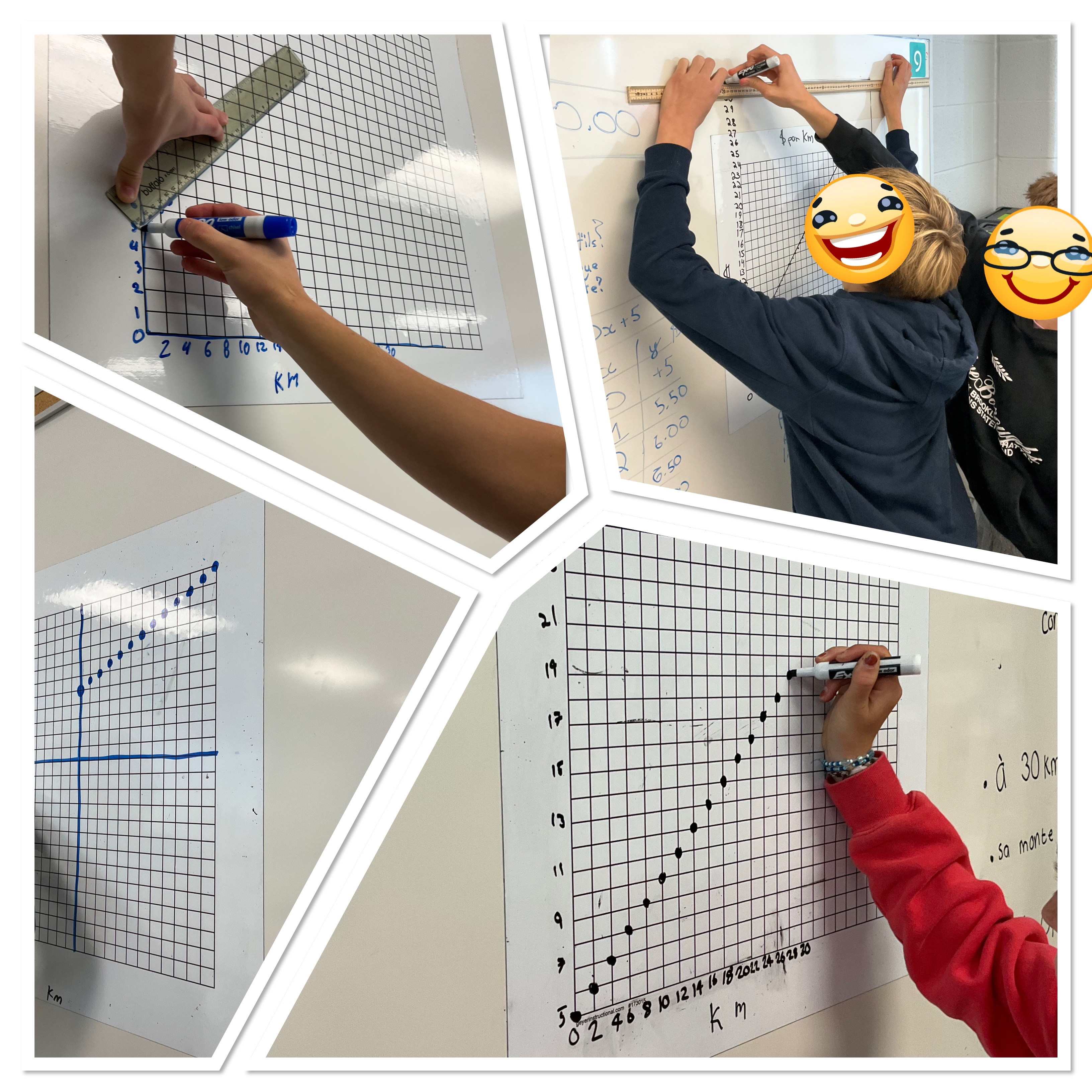
After graphing and making equations, they were given an extension question: if you have $30 how far could you travel?
Graphs were extended, tables were extended, equations were solved and we all agreed on an answer. The final video, for Act 3 is here. It shows the answer to the question posed in the 2nd video.
Our 2nd 3 act task was “Fast Clapper”.
here is the act 1 video which we watched, then noticed and wondered. We decided we needed more information to see if he would break the posted record or not.
The act 2 video shows a counter on the screen which helps us do some calculations to solve the problem.
Some groups found out how many seconds it takes for 1 clap, then used that to figure out how many claps he can do in 1 second, and then in 60 seconds.

This group found that he could do 63 claps on 4.6 seconds, which they said was about 4.5 seconds, and that 4.5×13.33 equals 60, so 63×13.33 would be the number of claps. Great use of proportional reasoning. They knew that they were over estimating since they used 4.5 instead of 4.6 seconds.

This group extended a table, counting by 5 second increments to figure out how many claps there’d be in a minute. They were showing that they understood the use of proportions and rate. There would be 5 times as many claps if we have 5 times as many seconds.

Lots of our work hinged on the idea that the rate stayed the same the whole time. We were not sure if he’d slow down or speed up during the minute, but that would also affect our calculations.
here is the act 3 video with the final reveal
We then wanted more information so we looked up to see if he is still the fastest clapper in the world. (Spoiler alert: he is NOT!)
Here’s a video about the current fastest clapper
Similar Triangles
We built triangles today out of pattern blocks. We looked at how the side lengths scale. The single triangle has a side length of 1, and an area of 1 triangle. We can see that the triangles in the photo have side lengths of 2, 3, and 4, and they have areas of 4 triangles, 9 triangles and 16 triangles.
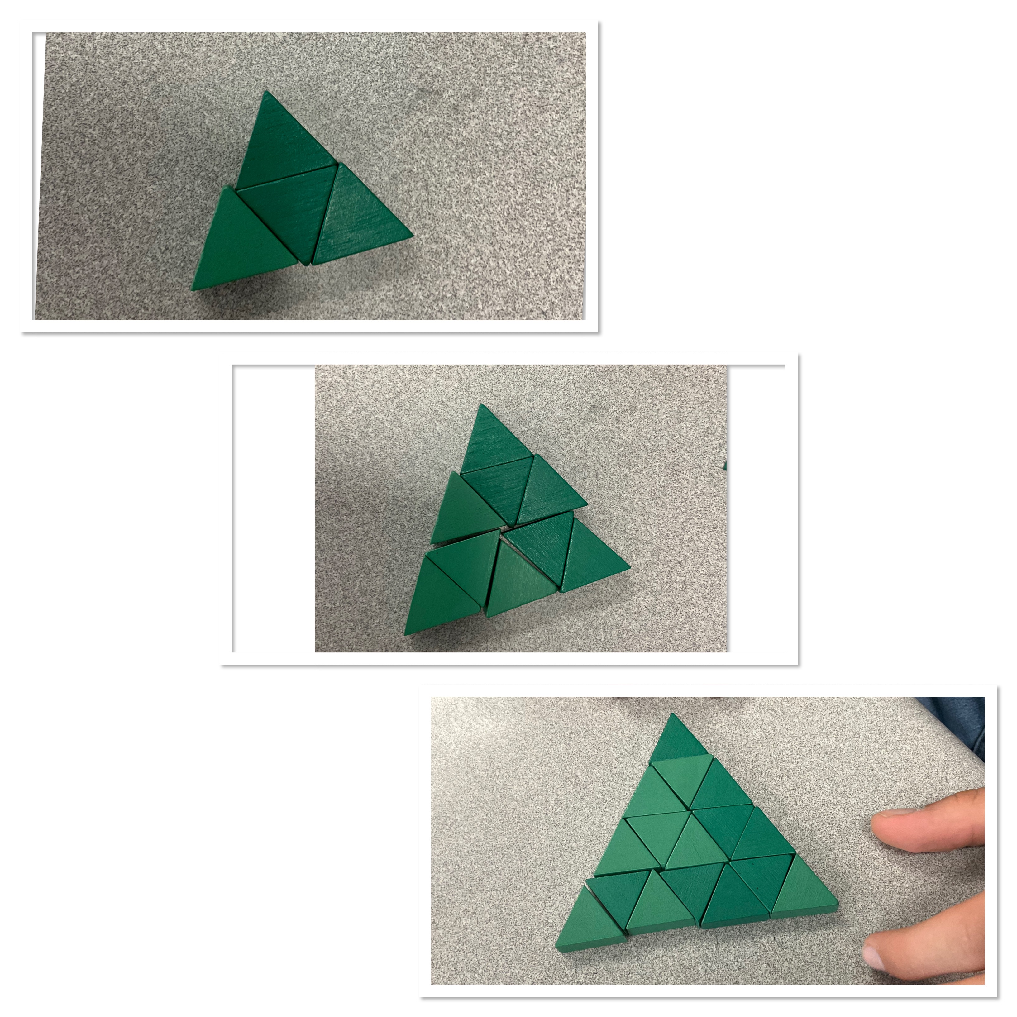
We made the inference that if we built a triangle that had a side lengths of 5 that it’d take 25 triangle tiles to do it.
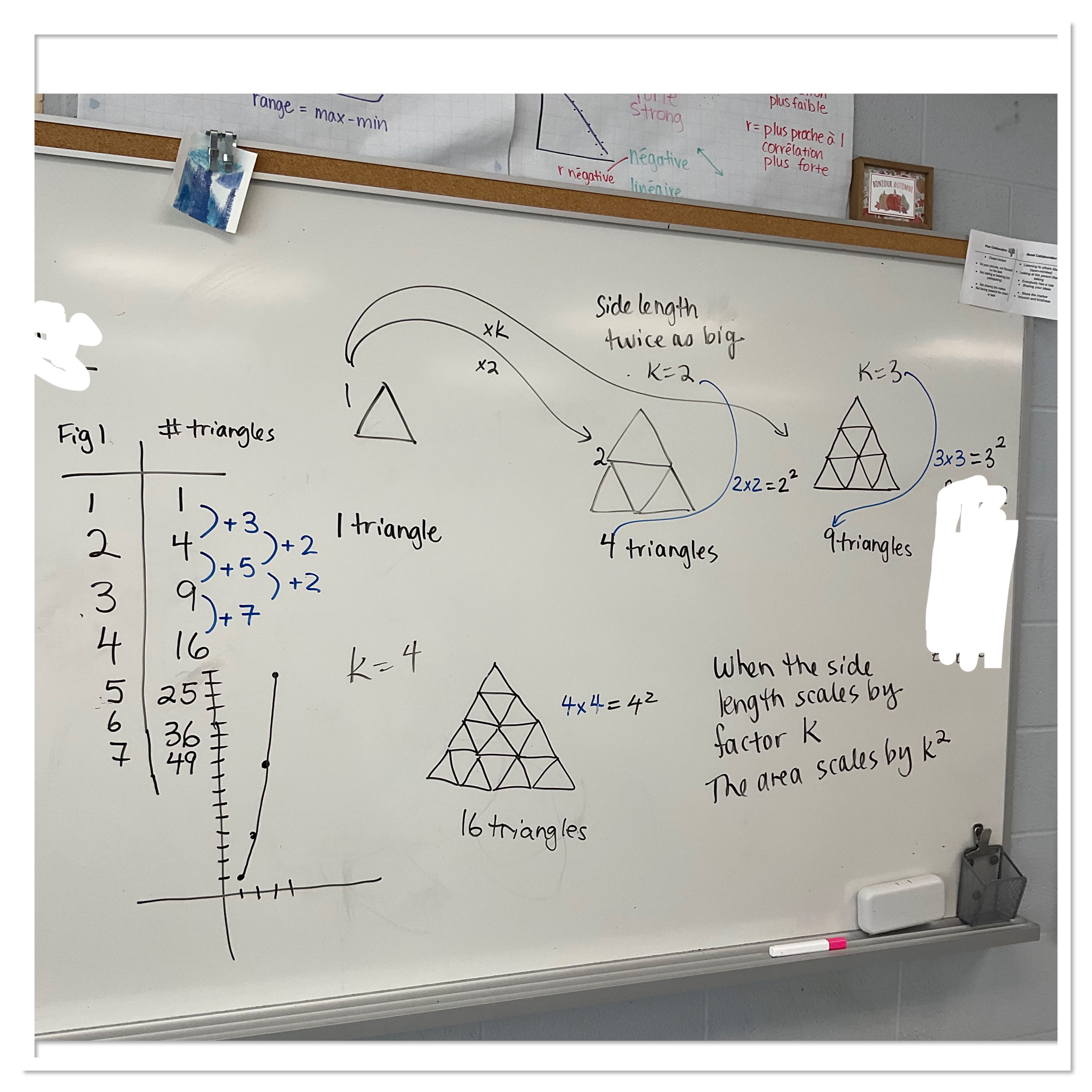
We consolidated the idea that if a side lengths scales by the factor k, the area will scale by the factor k squared. We noticed that this connects beautifully to our quadratic patterning that we had been looking at, with a second difference being the same each time, and a graph that is a curve, and the equation would be y=x^2 so there’s an exponent of 2 which indicates that the relationship is quadratic.
Graphing Lines using Visual Patterns
Today in grade 9 we started graphing lines. We used our skills in visual patterns to help us out. Each group got a pattern rule and 1 inch square tiles to build the pattern. We needed figure 0, figure 1, figure 2, figure 3, figure 4 at least.
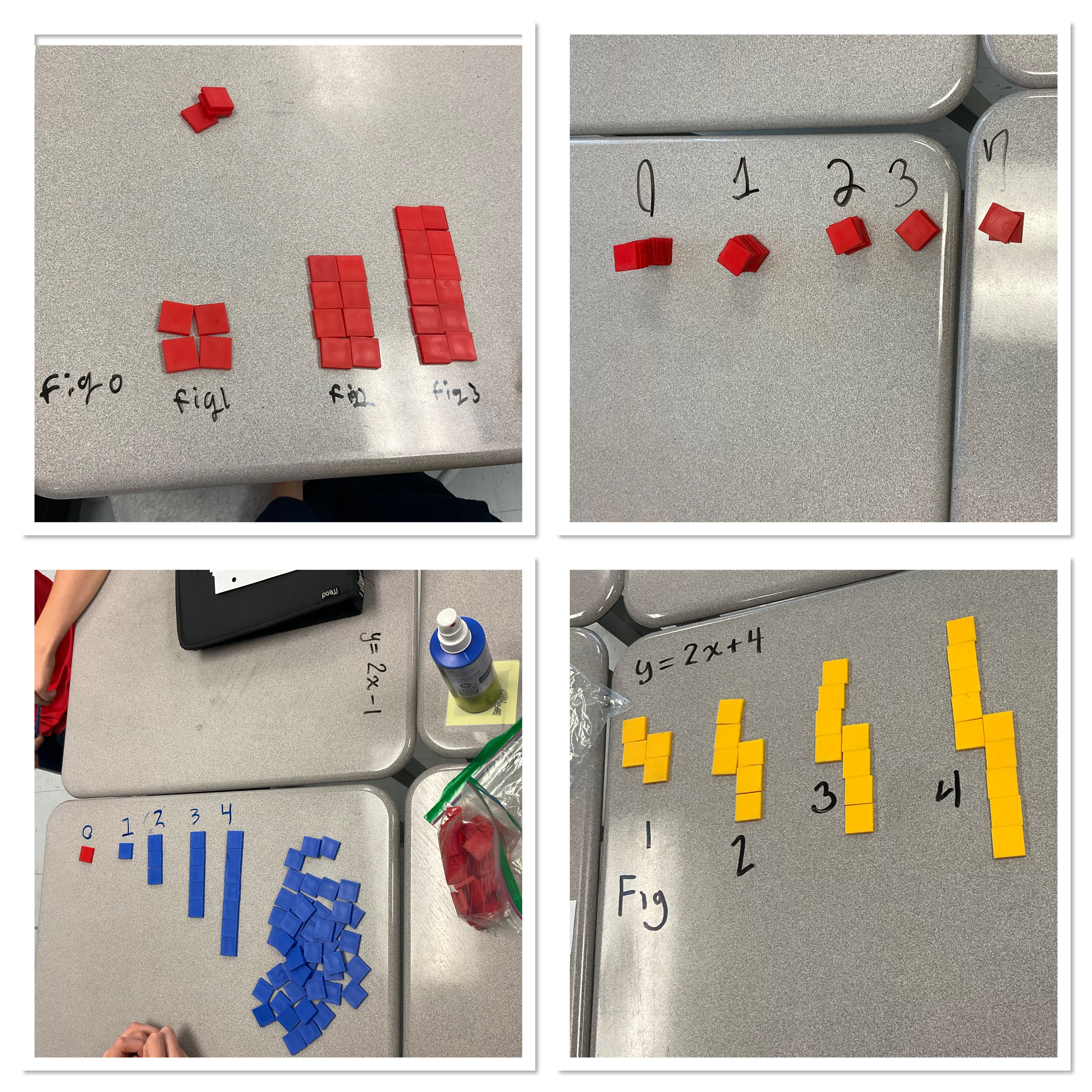
Next groups used 1” grid chart paper with x ans y axes drawn on it. They carefully moved all the tiles from figure 0 into a column on the graph paper that lined up with the y axis. They drew a dot at the top left of their column. The next figure was then dismantled and rebuilt into a column beside figure 0. A dot was placed at the top left. This was repeated until all of their figures had been moved and traced.
Next the dots were connected to form the line. Groups were given a different pattern rule and we did the same steps making a second graph superimposed on the first.

Finally we put them on the wall and then did some consolidation from our examples.
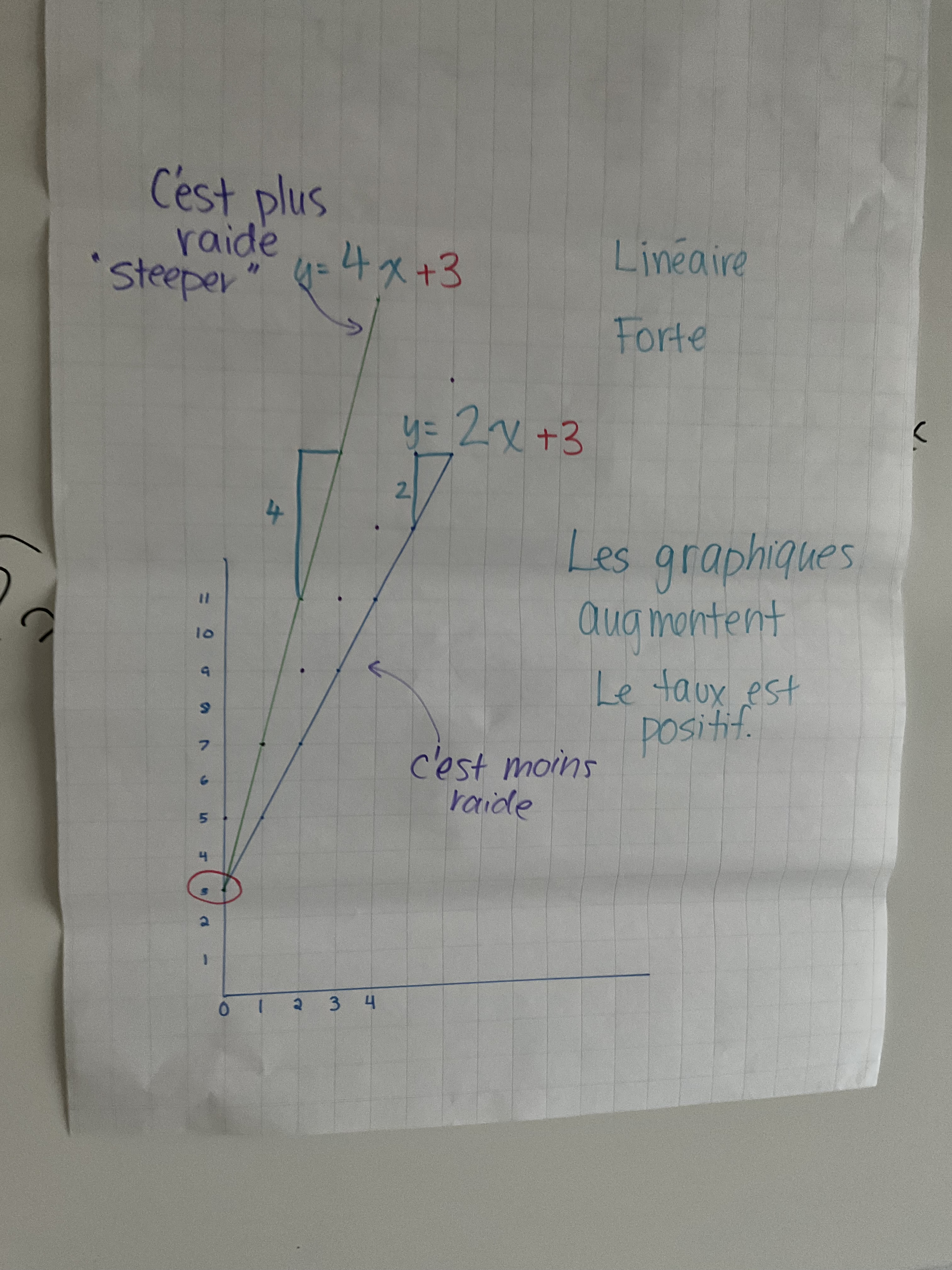
We identified parallel lines, how they have the same slope and will never intersect. We noticed that the slope is the number in front of the x, that multiplies the x. That’s also the rate of change. In French, le taux, la pente. We noticed that the constant will give us the y intercept on our graph.

We looked at slopes that were steeper and less steep. We noticed that the bigger the value for the slope, the more the line increases each time. We saw that if the equation was just y=4x that the constant is 0, and the line crosses the y axis at the origine (0,0). Here there is an intersection point at (1,4).

This graph shows a line with a positive slope of 2, and a line with a negative slope of -1. We noticed that the equation can be written like y=2x-1 or y=4-x, the constant could come first or last. We noticed that the constant represents where the graph crosses the y axis, even when it’s a negative number, so we needed to extend the axis down to accommodate it. We estimated the intersection point here. There’s a way to calculate it, but we’re not there yet.

Here we have 2 negative slopes, representing decreasing patterns. There is an intersection point, which is also called the solution. We can draw slope triangles to see the rise and run and visualize the slope.

We noted that it’s possible for a system of equations to intersect 0 times if the lines are parallel and distinct, 1 time if the slopes are different, and infinite times if the two lines are the same exact lines.
We finished off the class watching some excellent videos
Hopefully this summary helps those who were away at leadership camp get caught up!
Non-linear patterning
In grade 9 we were exploring linear and non-linear patterns. We had to decide if this pattern is linear or non-linear.

Students knew that the patten works by adding one each time, so the pattern rule is y=1x+3.
There was a lot of discussion about this next pattern. Some saw it as linear, where we’d add 7 each time.
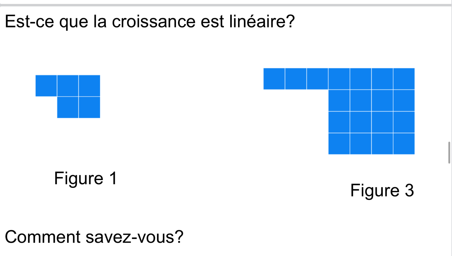

This would continue as follows, adding 7 each time…but with a few more figures people decided that the vibes were off, and the visual pattern didn’t look right.

so maybe it’s not linear.
we explored the growth in a few ways. We can see it as a big square (the green square) which is always one bigger than the figure number…or (x+1)^2. Plus we need one group of the figure number. Y=(x+1)^2+x.

We could also see a yellow x^2 and 3 groups of x and 1. Y=x^2+3x+1
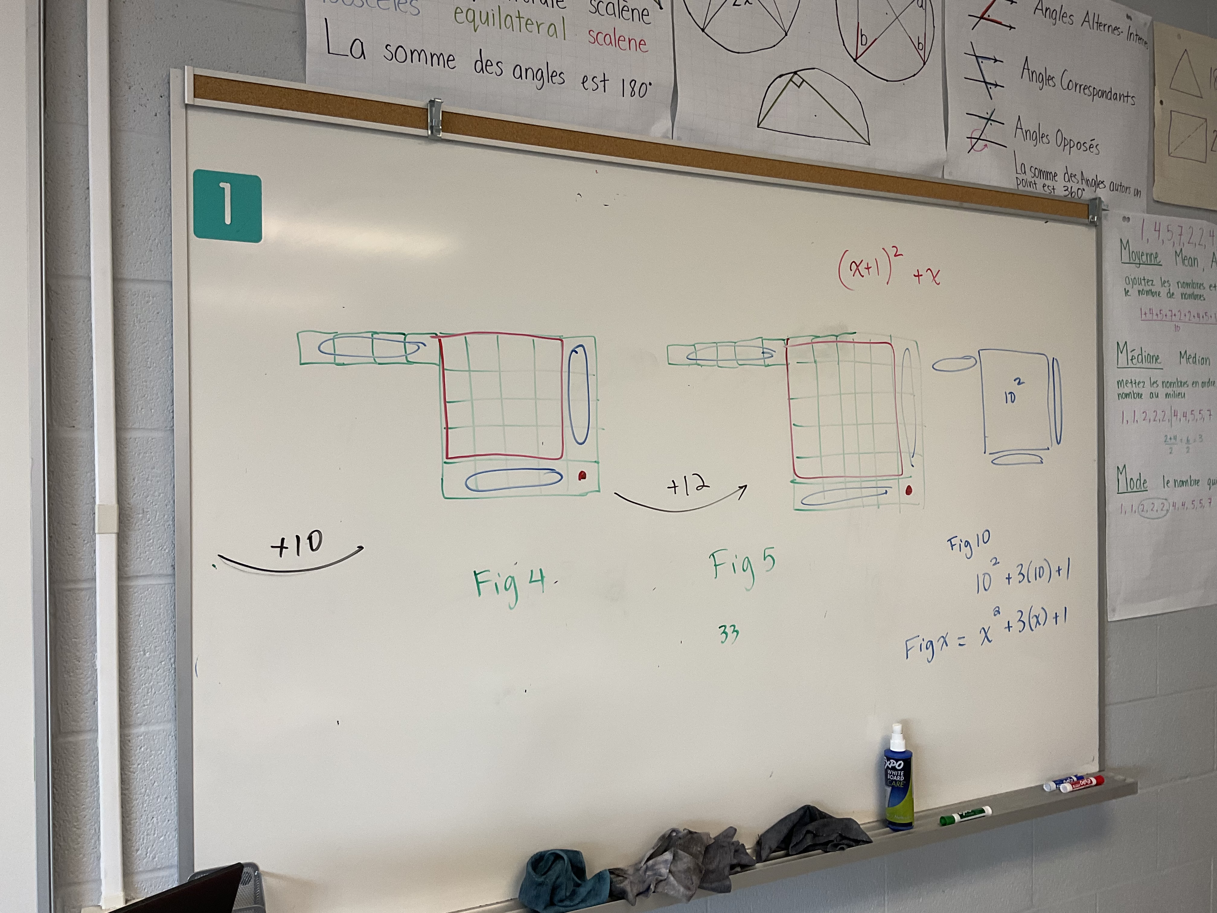
This pattern works much better in the long run! We know it’s not linear because we add a different amount each time.
Knot Tying Task
I was invited to join a grade 10 class today to try out the knot tying task I had done a few weeks ago. This time through it was with an academic class, so we added more algebraic aspects to the investigation.

Each group chose 2 ropes. There were longer thicker ropes and shorter thinner ropes and shortest thinnest ropes. They measured the ropes to start with, then tied a knot, then measured, then tied a knot then measured until 10 knots were tied.
They made graphs of their data, made lines of best fit for their data and then made the equations for the lines of best fit.
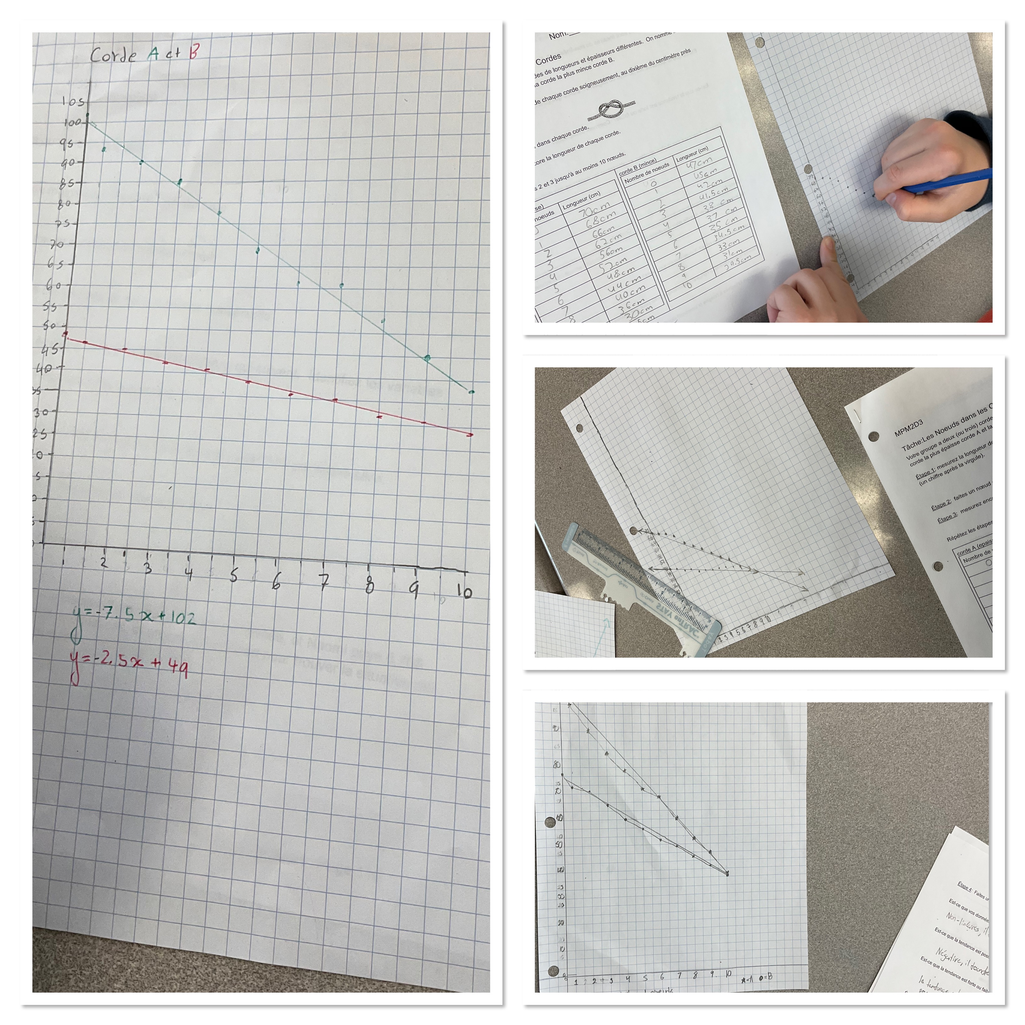
They needed to determine if there was a number of knots that would make both ropes the same length. This could be solved graphically, but we wanted them to practice their new skill of substitution, so they substituted to solve for the intersection point.
We consolidated in the middle about how to draw a line of best fit, then again a bit later we consolidated how to find the slope and y intercept of this line.
At the end the consolidation mostly focused on what the solution to the system meant, and why it made sense to do substitution. We know that the x represents the number of knots and the y represents the rope length. If we want to know when the ropes are the same length we set the y values equal. That means that the mx+b parts of the equations are also equal. We can solve for the x that makes this true (which represents the number of knots associated with the intersection point). Then we figure out the length of rope associated with that many knots by substituting back into the rope length equation.
It was neat to see lightbulbs go off when students recognized that each knot was shrinking the ropes by approximately the same amount each time, and that the rate of change of the rope length per knot was the slope, and the initial rope length was the y intercept. Having a context to connect the ideas to was really helpful for many students. I look forward to trying this task with another group.
